In a previous post I promised to explore how we can use the statistics package R to produce estimates for the relative proportions of Republicans, Democrats, and unaffiliated and other voters within the total population voting in the 2010 general election. However I spent all of last post on the preliminaries: how to download and install R, and how to load into R turnout data from past Howard County gubernatorial primary and general elections. In this post we can start doing some real work.
First, let’s restart R and make sure we have the data we’ll be using. If you told R to save your workspace at the end of your last session, then R should automatically restore that workspace, including the turnout data, when you start it now:
R version 2.12.0 (2010-10-15)
Copyright (C) 2010 The R Foundation for Statistical Computing
ISBN 3-900051-07-0
Platform: i386-apple-darwin9.8.0/i386 (32-bit)
...
[Workspace restored from /Users/hecker/.RData]
[History restored from /Users/hecker/.Rhistory]

>
If you didn’t save your workspace, or if R doesn’t restore it for some reason, then you can reload the data following the instructions in the last post. Either way, when you’re done you should have two variables (“data frames”) that contain the data of interest, hgp for the primary election turnout data and hgg for the general election turnout data. You can use the ls() command to verify that the variables are present, and enter the variables’ names to print their values (here I show the data in the data frame hgp):
> ls()
[1] "hgg" "hgp"
> hgp
  Year Registered Turnout PctTurnout  RegD PctRegD TurnoutD PctTurnoutD
1 1990      92801   22989      24.77 47586   51.28    15001       31.52
2 1994      89492   37408      41.80 51949   58.05    23255       44.77
3 1998     128935   34066      26.42 61358   47.59    18219       29.69
4 2002     156505   39989      25.55 73240   46.80    23837       32.55
5 2006     161922   41324      25.52 75592   46.68    27984       37.02
   RegR PctRegR TurnoutR PctTurnoutR RegOther PctRegOther TurnoutOther
1 33923   36.55     7675       22.62    11292       12.17          313
2 37543   41.95    14153       37.70    14598       16.31          656
3 47019   36.47    15218       32.37    20558       15.94          629
4 56409   36.04    14719       26.09    26856       17.16         1433
5 55045   33.99    12036       21.87    31285       19.32         1304
  PctTurnoutOther PctVotersD PctVotersR PctVotersOther
1            2.77      65.25      33.39           1.36
2            4.49      62.17      37.83           1.75
3            3.06      53.48      44.67           1.85
4            5.34      59.61      36.81           3.58
5            4.17      67.72      29.13           3.16
>
OK, can we start estimating now? Not so fast. . . . Let’s first devote a bit of thought to what we’re trying to estimate, and what general approaches we might use to do it. Recall that our previously-stated goal was to estimate the relative proportions of Democrats, Republicans, and unaffiliated and other voters voting in the 2010 general election. Why these particular values? Because they are typically used in political polling when constructing a sample of likely voters. Obviously polling a sample consisting of 90% Democrats would produce a biased result, as would polling a sample consisting of 75% Republicans or 50% independents.
So we want to estimate three separate values for the 2010 general election: the proportion of those voting who are registered Democrats, the proportion of those voting who are registered Republicans, and the proportion of those voting who are unaffiliated or belong to other (smaller) parties. Note that by definition these three values must add up to 100%; therefore we need only estimate two of them, and then we can compute the third estimate by taking the sum of the first two estimates and subtracting it from 100. (For example, if we estimate 50% Democrats and 40% Republicans then the estimated number of independents is 100% minus 90% or 10%.)
How might we go about estimating these values? Assuming we’re not just going to use our gut (“feels like a tsunami this year”) we should try to use the data that’s available to us. But what data? In our case we have in essence four separate data sets: turnout data for primary elections in presidential years, data for gubernatorial primaries, and turnout data for general elections in both presidential election years and gubernatorial election years.
I’ve already made one decision about which data to use, namely to focus only on data from gubernatorial elections, on the theory that turnout patterns in presidential election years are different enough that they aren’t necessarily a good guide for estimating turnout in gubernatorial election years. (For example, turnout tends to be significantly higher across the board in presidential election years.)
We now face a second choice: Should we use only the general election data, only the primary election data, or both? For example, it might be the case that turnout in a primary election predicts fairly well turnout in a general election; we could try to dermine some sort of relationship between primary and general election turnout using data from previous years, and then use the primary turnout data from 2010 to estimate the turnout for the 2010 general election. An alternative theory is that there’s not a strong relationship between turnout in primaries and turnout in general elections, in which case we should focus solely on general election data. Finally, it might be that general election turnout in 2010 is a function of both 2010 primary election turnout and general election turnout in prior years.
I’ll start the same way I originally started, and look at general election data only. (We can then come back and look at the primary data later.) But we’ve still got the problem of deciding exactly which variables to look at: Absolute numbers of registered voters in past general elections? Relative percentages of registered voters among the parties and independents (e.g., what percentage of registered voters are Democrats)? Relative turnout between the parties (e.g., what percentage of registered Democrats actually voted vs. what percentage of Republicans voted)? And so on. As seen in printing out hgg and hgp, we have 19 different columns of data we can play with, representing results from five different elections.
The simplest approach is to look first at the historical data for the quantities we’re trying to estimate, and see if there are any discernible trends. In our case that means looking at the three variables hgg$PctVotersD (percentage of those voting in general elections who are registered Democrats), hgg$PctVotersR (percentage of those voting in general elections who are registered Republican), and hgg$PctVotersOther (percentage of those voting in general elections who are unaffiliated or are registered members of other parties). Rather than applying any heavy statistical techniques, let’s just use R to plot the values of these variables over time.
I’ll start with the percentage of voters who are Republicans, as I did when I did my original analysis, and use the plot() command to plot the values of hgg$PctVotersR against the values of hgg$Year:
> plot(hgg$Year, hgg$PctVotersR)
>
R can generate very complicated and professional-looking plots, but in this case we get the following barebones but nonetheless useful graph:
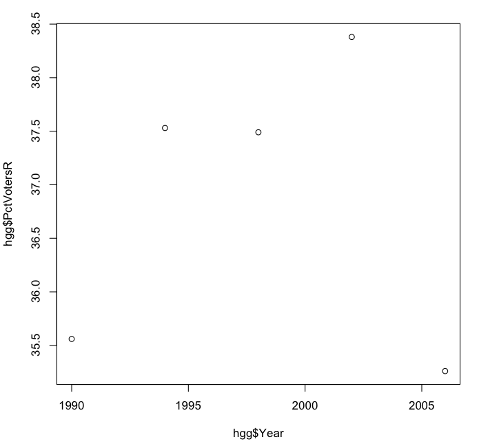
It’s hard to discern a trend here. It looks as if the percentage of Republican voters was rising from 1998 to 2002, only to drop off in 2006 to its original level. The vertical scale of the graph exaggerates the relative differences from year to year, so let’s redo the plot, this time using a vertical scale from 0 to 60 percent.
> plot(hgg$Year, hgg$PctVotersR, ylim = c(0, 60))
>
Here the ylim parameter sets the range of values on the vertical (“y”) axis to 0 on the low end and 60 on the high end. The value c(0,60) is a list of two numbers (a “vector” in R terminology) concatenated together (where the “c” comes from).
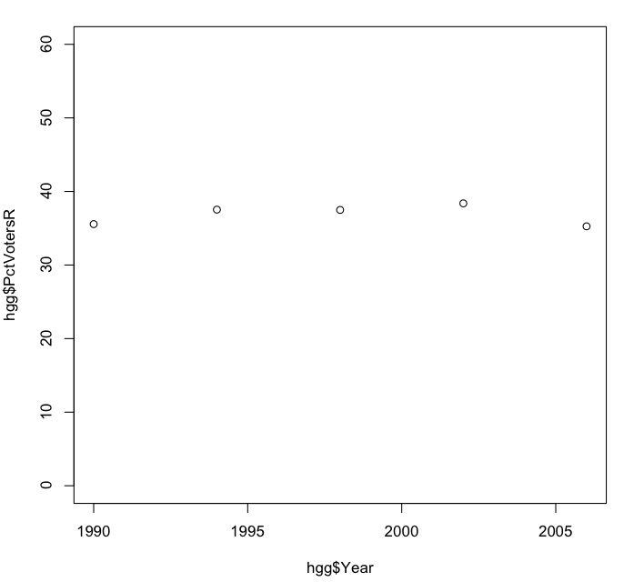
Notice that in this plot the percentage of Republican voters appears relatively static, fluctuating somewhere between 35% and 40% over the years. We can get a bit more specific about this by computing the mean and standard deviation of these values:
> mean(hgg$PctVotersR)
[1] 36.844
> sd(hgg$PctVotersR)
[1] 1.360599
>
The mean of 36.84% is what’s more commonly known as the average: the sum of all the percentages of Republican voters in the five gubernatorial elections, divided by the number of elections. The exact computation of the standard deviation of 1.36% is not important for our purposes; we can use it simply as a measure of how tightly or loosely the various values are clustered about the mean. (If you’re interested in how standard deviation is computed, see the relevant section of the associated Wikipedia article, and note that what R computes is what is technically known as the sample standard deviation.)
If the percentage of Republican voters from election to election were truly fluctuating randomly in a certain way (in statistical terms, if it were a random variable with a known distribution, e.g., a normal distribution) then we could use the mean and standard deviation together to make relatively strong predictions about the likely value of the Republican percentage of the vote in 2010. For example, we could define a 95% confidence interval like those we discussed in relation to polling margins of error, i.e., a range of values around the mean value, with only a 5% likelihood that the Republican percentage of the vote would fall outside that range.
In this case we don’t know whether we’d be justified in making such predictions or not. However it was this computation that originally made me somewhat skeptical of the Republican percentage of the vote going much above 40% (or much below 35%, for that matter). Whether that skepticism will be borne out remains to be seen. In the meantime I’ll end this post and take a break from R for a while; in the next post I’ll plot the historical percentages of the vote from Democrats and unaffiliated and other voters, and see if they show any clearer trends.